Visualization
spacedeconv_visualization.Rmd
To introduce spacedeconvs visualization functions we will utilize a
deconvolution result obtained from the sample data provided and the
deconvolution method spatialdwls. First we compute a
reference signature based on the available scRNA-seq data with
cell-type annotation. Then we quantify cell-type fractions in the
10X Visium slide using the computed reference signature.
library(spacedeconv)
data("spatial_data_3")
data("single_cell_data_3")

single_cell_data_3 <- spacedeconv::preprocess(single_cell_data_3)
spatial_data_3 <- spacedeconv::preprocess(spatial_data_3)

spatial_data_3 <- spacedeconv::normalize(spatial_data_3, method = "cpm")

signature <- spacedeconv::build_model(
  single_cell_obj = single_cell_data_3,
  cell_type_col = "celltype_major",
  method = "spatialdwls", verbose = T
)
## class of selected matrix:  dgCMatrix
## [1] "finished runPCA_factominer, method == factominer"
deconv <- spacedeconv::deconvolute(
  spatial_obj = spatial_data_3,
  single_cell_obj = single_cell_data_3,
  cell_type_col = "celltype_major",
  method = "spatialdwls",
  signature = signature,
  assay_sp = "cpm"
)
## class of selected matrix:  dgCMatrix
## [1] "finished runPCA_factominer, method == factominer"
Available Visualizations
-
plot_spatial()generates a Hex Plot of a SpatialExperiment containing deconvolution results. -
plot_gene()plot spatial gene expression. -
plot_umi_count()Plots the number of sequenced reads per spot. -
plot_most_abundant()Render a plot containing the most abundant cell-type for each spot. -
plot_comparison()Plot comparison of two cell-type fractions.
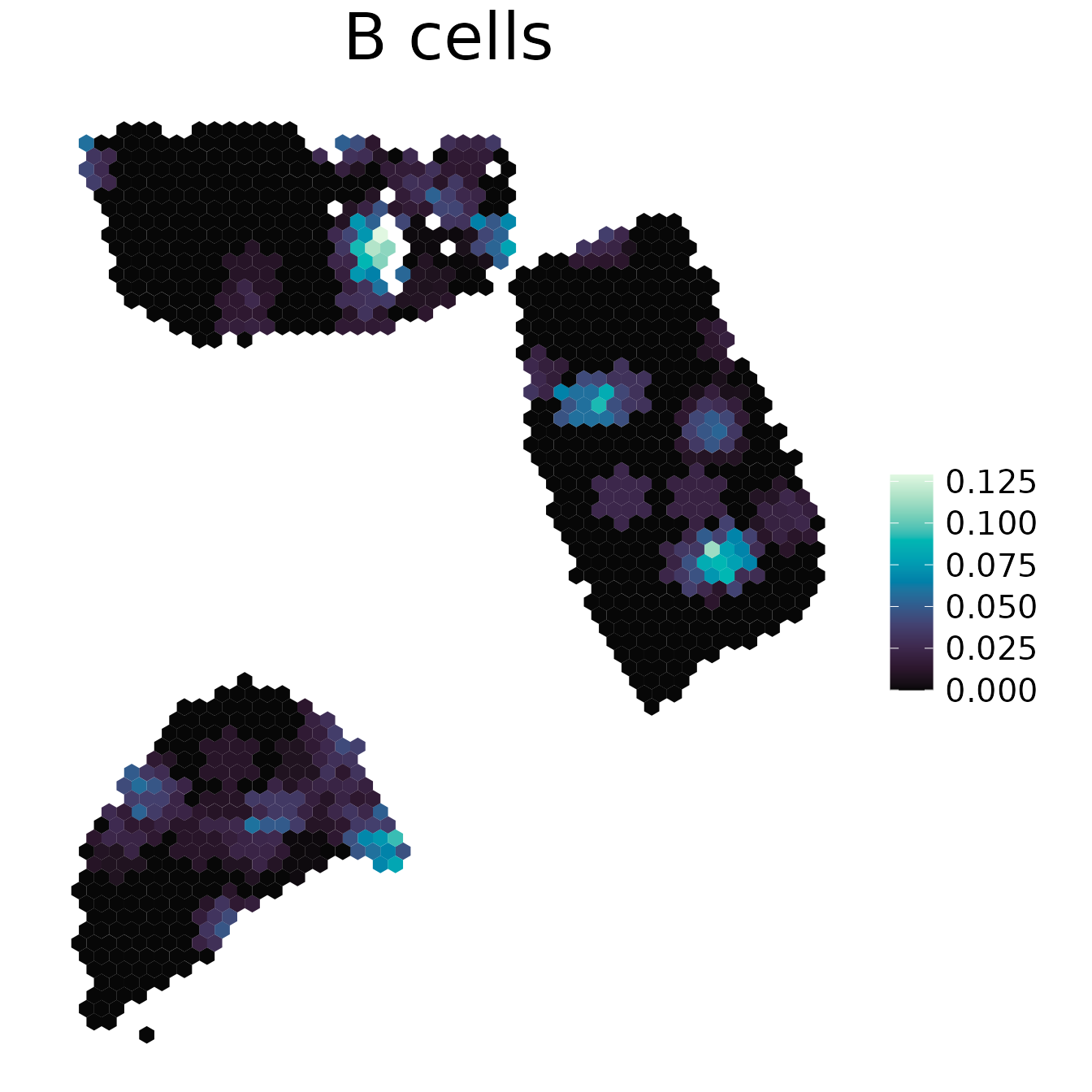
1. plot_spatial()
Plot any spot annotation with a continuous or discrete scale.
The spot annotation needs to be of colData(spe), so
manual annotation can be added to the SpatialExperiment object
for visualization.
spacedeconv::plot_spatial(deconv, result = "spatialdwls_B.cells", density = F, smooth = T, title="B cells")
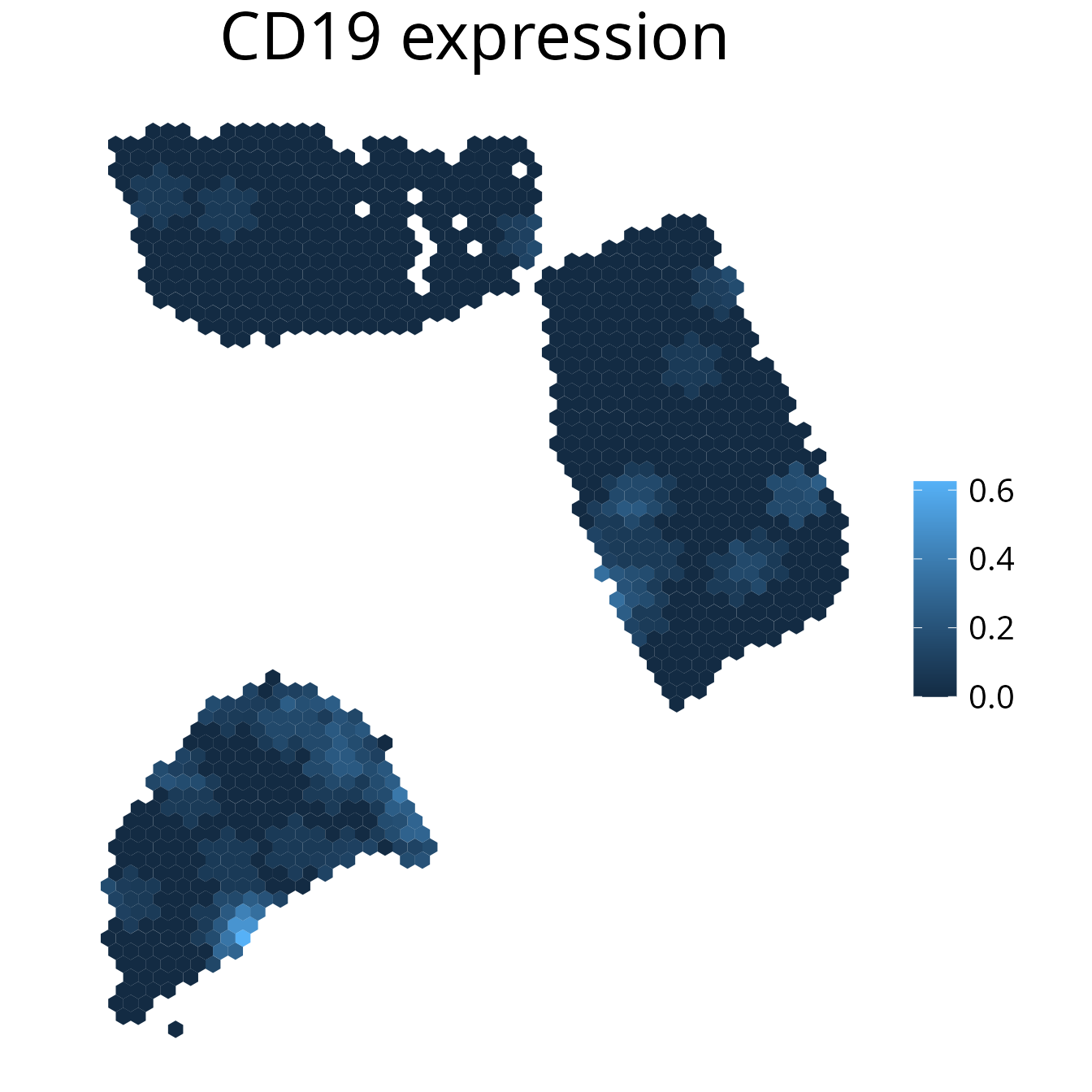
2. plot_gene()
Plot gene expression on a spatial level. It may make sense to
smooth the plot to simplify the detection of expression
patterns. You can further select the assay using the
assay parameter.
spacedeconv::plot_gene(deconv, gene = "CD19", density = F, smooth = T, title_size=12)
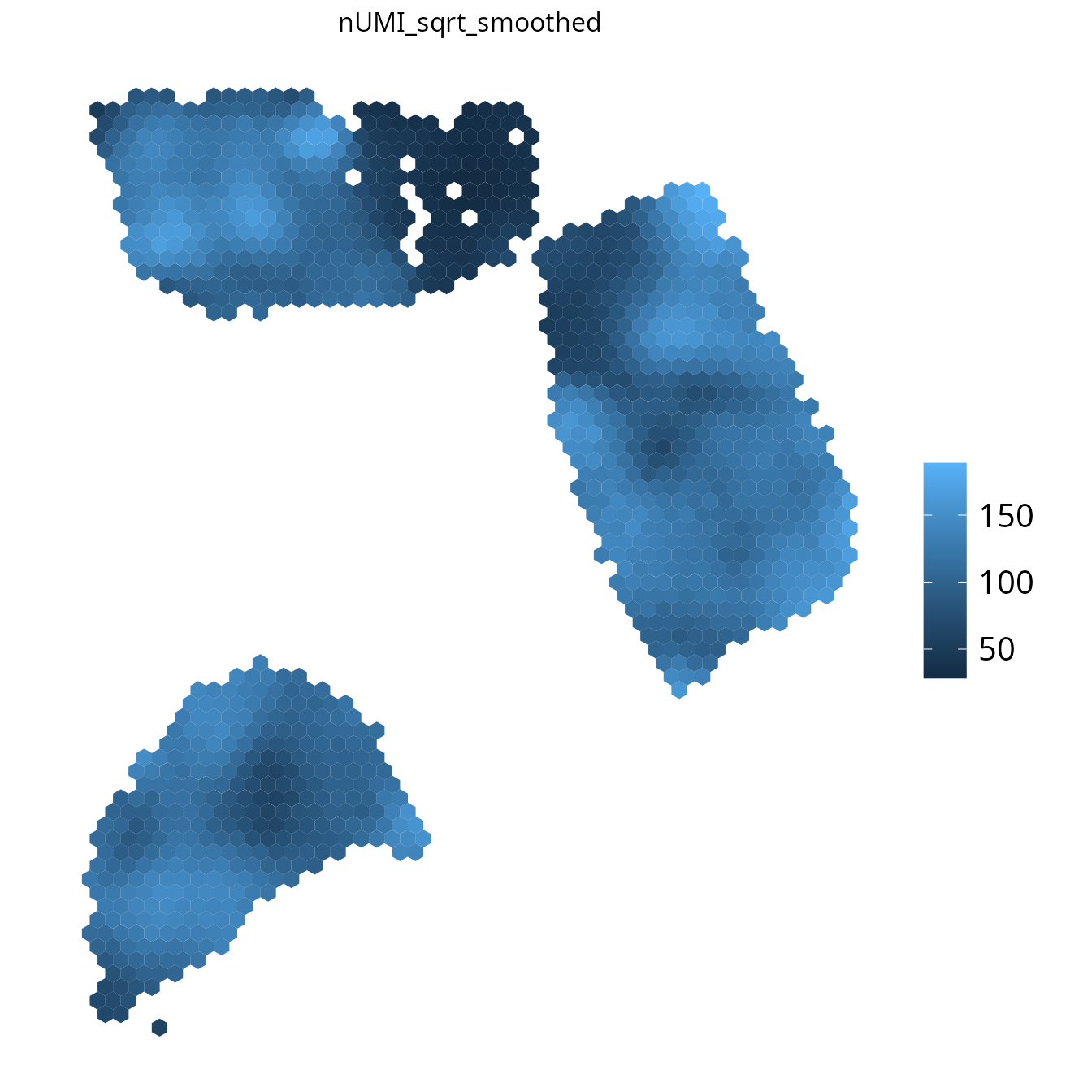
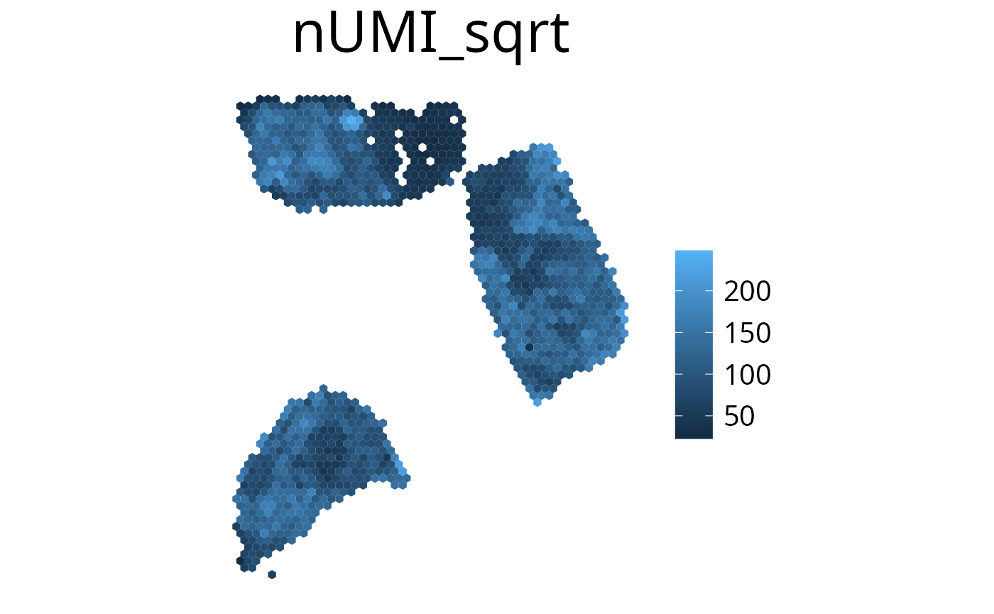
3. plot_umi_count()
This plot shows the number of detected UMIs for each spot. We
recommend rendering this plot with
transform_scale = "sqrt" due to the large range of
UMI count values.
spacedeconv::plot_umi_count(deconv, transform_scale = "sqrt", density = F, smooth = T, title_size=12)
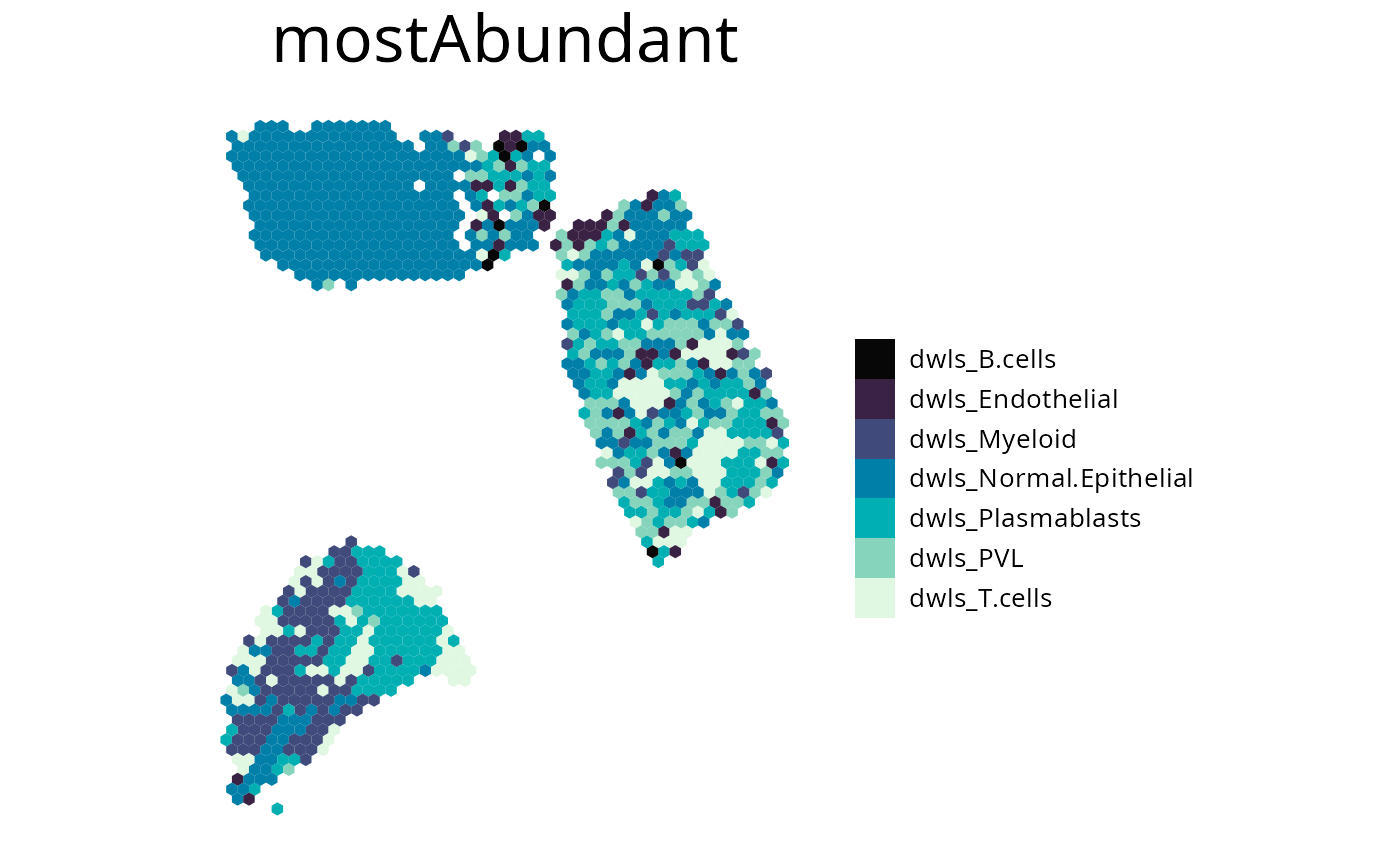
4. plot_most_abundant()
This plots displays the most abundant cell-type for each spot. You can specify which cells to plot by either one of the following:
cell_typevector of celltypes to plot-
methodplotting all cell types of the provided method -
removevector of celltypes to be removed from the plot
spacedeconv::plot_most_abundant(deconv,
  method = "spatialdwls",
  density = F,
  title_size = 12,
  legend_size = 15,
  font_size = 10,
  remove = c("spatialdwls_Cancer.Epithelial", "spatialdwls_CAFs")
)
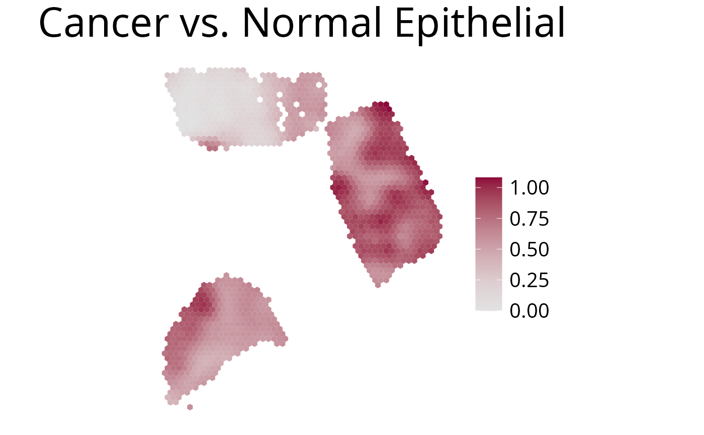
5. plot_comparison()
Use this function to plot the ratio of deconvolution results from two cell-types.
spacedeconv::plot_comparison(deconv,
  cell_type_1 = "spatialdwls_Cancer.Epithelial", # red
  cell_type_2 = "spatialdwls_Normal.Epithelial", # blue
  palette = "Blue-Red",
  density = F,
  smooth = T,
  title_size=12
)
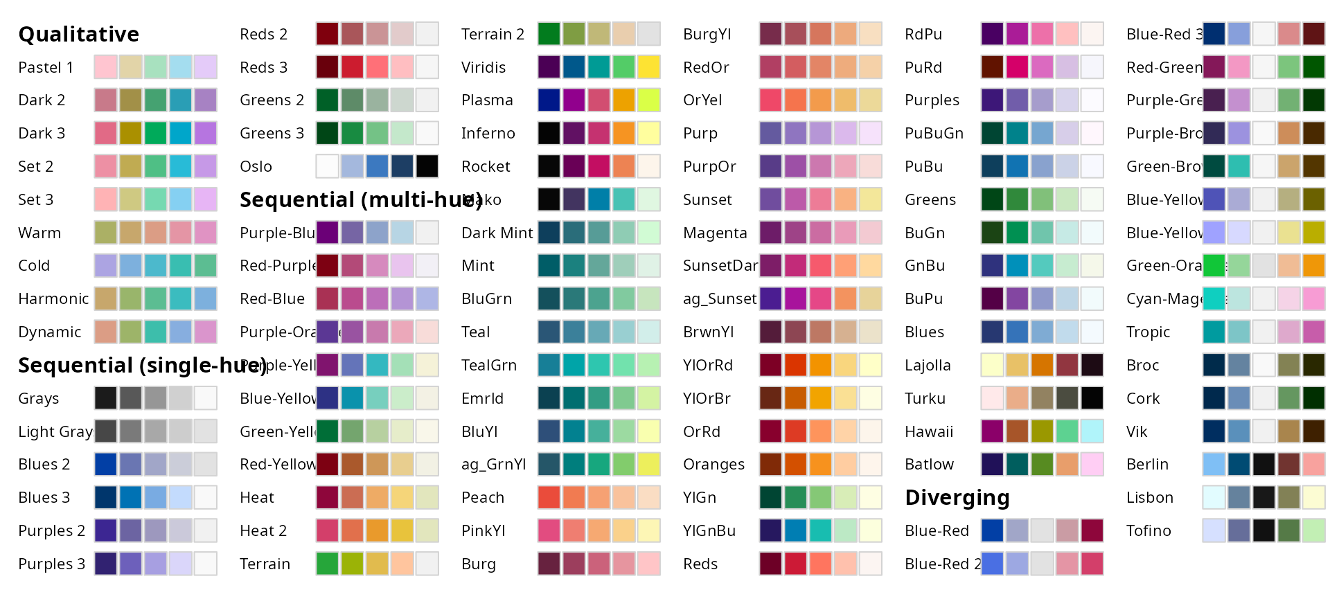
Color Palette
All palettes from the colorspace R Package can be used.
colorspace::hcl_palettes(plot = TRUE)
Further plot adjustments
Image Alignment Offset
spacedeconvs Visualization function is designed to work with
data by SpaceRanger >= V2.0. Since this Version the image is
rotated by default that the hourglass fiducial is in the upper
left corner. Previous SpaceRanger results can be rotated
differently. The rotation additionally reflects in the angle of
the spots on the slide. Uncorrectly rotated images result in
hexagons being rotated by 30 degrees. To compensate for this you
can use the offset_rotation parameter to correct
the hexagon alignment. This is only necessary for Visium slides
where the hourglass fiducial is in the bottom left or upper
right corner.
plot_umi_count(deconv, offset_rotation = T, title_size=12) # rotate hexagons

Transform Scale
With the transform_scale parameter the colorspace
scale can be modified. Available options are: “ln”, “log10”,
“log2” and “sqrt”. Scaling the color range differently can aid
with interpreting the plot. Please have in mind that the plot
does not show valid deconvolution results anymore and should be
handled with caution.
spacedeconv::plot_umi_count(deconv, transform_scale = "sqrt", density = FALSE, title_size=12)
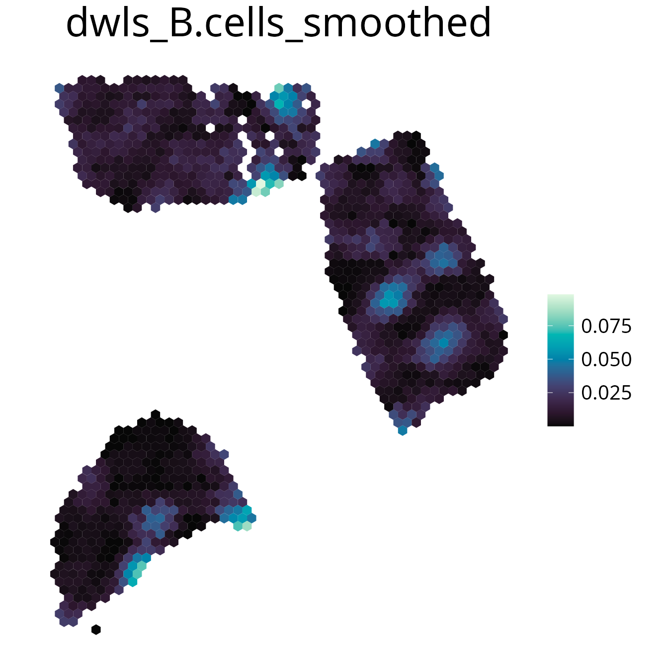
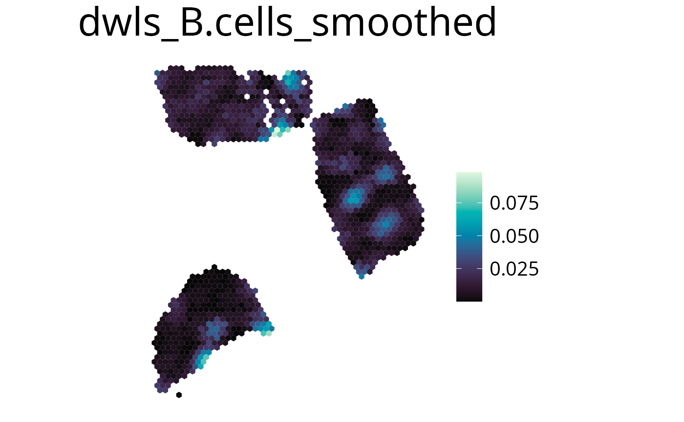
Smooth
With this parameter the expression values can be smoothed to simplify pattern recognition. The smoother utilizes a linear kernel which size is calculated by multiplying the spot distance with the smoothing factor. It has to be mentioned that this operation changes the deconvolution result in the final plots by appling the kernel, so they should be interpreted as a helpful visualization option and not a deconvolution result.
smooth=Tenable smoothing-
smoothing_factorchoose kernel size (factor of spot distance)
spacedeconv::plot_spatial(deconv,
  result = "spatialdwls_B.cells",
  smooth = T,
  smoothing_factor = 1.5,
  density = FALSE,
  title="B cells smoothed"
)
Density Distribution
You can add a density distribution by setting
density = TRUE. The red line corresponds to the
mean of the distribution.
spacedeconv::plot_spatial(deconv,
  result = "spatialdwls_B.cells",
  smooth = TRUE,
  density = TRUE,
  title="B cells with density"
)
Save Plots
You can save a plot by setting save=TRUE. Specify a
file path with the path parameter. If no path is
provided your plots will be stored at
~/spacedeconvResults/. To change the size of the
rendered plot use png_width and
png_height to set the plot size in pixels. Plots
are saved as a png.
spacedeconv::plot_spatial(deconv,
  result = "quantiseq_B.cell",
  smooth = TRUE,
  density = TRUE,
  save = TRUE,
  path = "~/project/results",
  png_width = 1000,
  png_height = 750
)
Aggregate cell types
Aggregate cell types using the aggregate function.
Internall the deconvolution results are summed up and get a new
name. The aggregation can be visualized with all available
plotting functions.
spe <- aggregate(spe, cell_type_1, cell_type_2, newName)
Additional Parameters
-
show_imagelogical, show or remove the spatial image -
spot_sizeinteger, increase (>1) or decrease (<1) the hexagon size -
limitsvector containing upper and lower limits for the color scale -
palette_type“discrete”, “sequential” or “divergent”, how to scale the color´ reverse_palettereverse color palettefont_sizefont size of legendtitle_sizefont size of titlelegend_sizelegendtitleset a custom title