Deconvolution of the tumor microenvironment with omnideconv

1. Introduction and dataset

In this vignette, we will use the omnideconv package to deconvolve a bulk RNA-seq dataset from 24 breast cancer patients with two different methods (DWLS and BayesPrism). The datasets are from a recent breast cancer study (Wu et al. 2021). This study provides access to a primary-tumor single cell RNA-seq (scRNA-seq) dataset from 26 breast cancer patients across three major cancer subtypes (ER+, HER2+, TNBC). The dataset includes cell-type annotation for three resolution levels. In addition, the data includes bulk RNA-seq sequencing for 24 of the patients. In this chapter, we use multi-sample, breast-cancer scRNA-seq atlas (100,064 cells) as a reference to train the methods for the deconvolution of the bulk RNA-seq samples. The single-cell and bulk RNA-seq data is deposited on GEO, under accession number: GSE176078. The single cell data comes with the author’s cell type annotations. We will need to download and unzip the datasets (GSE176078_Wu_etal_2021_BRCA_scRNASeq.tar.gz, GSE176078_Wu_etal_2021_bulkRNAseq_raw_counts.txt.gz), and store them in a data directory. For this example analysis, we will also need the additional clinical information about the patients, available as Supplementary Table 1 from the paper.

2. Library loading

library(Seurat)
library(tidyverse)
library(omnideconv)
library(readxl)

3. Single cell data processing

Although not strictly required by omnideconv, we suggest performing quality control and filtering of the input scRNA-seq data according to the best practice (Heumos et al. 2023), to ensure the best training conditions for deconvolution algorithms. We first pre-process the single-cell dataset to remove low-quality cells. We will use the R package Seurat (Hao et al. 2023), which allows fast and easy manipulation of single-cell data. We will create a Seurat object with the cell counts and their metadata of interest curated by the authors, which include cell-type annotation on three levels of resolution:

single.cell.data <- Seurat::ReadMtx(
  mtx = "path/to/Wu_etal_2021_BRCA_scRNASeq/count_matrix_sparse.mtx",
  cells = "path/to/Wu_etal_2021_BRCA_scRNASeq/count_matrix_barcodes.tsv",
  features = "path/to/Wu_etal_2021_BRCA_scRNASeq/count_matrix_genes.tsv",
  feature.column = 1
)
single.cell.metadata <- read.table("path/to/Wu_etal_2021_BRCA_scRNASeq/metadata.csv",
  sep = ",", header = TRUE, row.names = 1
)

single.cell.data <- CreateSeuratObject(single.cell.data,
  project = "Wu_dataset", assay = "RNA",
  min.cells = 0, min.features = 1,
  meta.data = single.cell.metadata
)

We can have an overview of the number of cells per cell type in the dataset:

Number of cells per cell type

celltype_major	number_cells
B-cells	3206
CAFs	6573
Cancer Epithelial	24489
Endothelial	7605
Myeloid	9675
Normal Epithelial	4355
Plasmablasts	3524
PVL	5423
T-cells	35214

In order to remove low quality cells, we will follow the best practices for single cell normalization (Heumos et al. 2023). We will perform quality control on each cell by considering metrics such as the number of total counts, the number of expressed features (genes), and the fraction of mitochondrial genes per cell. We will remove cells that have $MAD = median(|X_i - median(X)|)$, where

• $X_i$ is the respective metric of an observation $i$ (cell), for example the number of detected genes
• $MAD$ is the Median Absolute Deviation, computed as $MAD = median(|X_i - median(X)|)$
• $n$ is set to 5 for the number of counts and expressed features, and to 3 for the fraction of mitochondrial genes

In order to do this filtering, we will create a function to identify the outliers for each metric:

is_outlier <- function(SeuratObject, metric, nmads) {
  eval(parse(text = paste0("M <- SeuratObject$", metric)))
  outlier <- (M < median(M) - nmads * mad(M)) | (M > median(M) + nmads * mad(M))
  return(outlier)
}

check_outliers_nFeature <- is_outlier(single.cell.data, "nFeature_RNA", 5)
check_outliers_nCount <- is_outlier(single.cell.data, "nCount_RNA", 5)
check_outliers_mito <- is_outlier(single.cell.data, "percent.mito", 3)

non_outliers_nFeature <- names(check_outliers_nFeature[!check_outliers_nFeature])
non_outliers_nCount <- names(check_outliers_nCount[!check_outliers_nCount])
non_outliers_mito <- names(check_outliers_mito[!check_outliers_mito])

non_outliers <- intersect(non_outliers_nFeature, non_outliers_nCount) %>%
  intersect(non_outliers_mito)

single.cell.data <- subset(single.cell.data, cells = non_outliers)

Number of cells per cell type after quality filtering

celltype_major	number_cells
B-cells	3150
CAFs	6154
Cancer Epithelial	16613
Endothelial	6991
Myeloid	8855
Normal Epithelial	3533
Plasmablasts	3164
PVL	5120
T-cells	34991

4. Bulk data preprocessing

We will now read in the bulk sequencing data file, which consists of 24 samples.

bulk.data <- read.table("path/to/GSE176078_Wu_etal_2021_bulkRNAseq_raw_counts.txt", skip = 1)
header <- read.table("path/to/GSE176078_Wu_etal_2021_bulkRNAseq_raw_counts.txt",
  header = FALSE, nrows = 1, skipNul = TRUE, sep = "\t"
)
colnames(bulk.data) <- c("Genes", gsub("A|N", "", header[2:25]))
bulk.data <- bulk.data[bulk.data$Genes != "", ]
bulk.data <- column_to_rownames(bulk.data, "Genes")
bulk.data <- as.matrix(bulk.data)

5. Subsampling of single cell data

The various methods included in omnideconv rely on the single cell dataset that will be used to train them for the deconvolution of those specific cell types. This training involves the optimization of internal features of the methods and can happen in different ways. Some methods use the single cell data to build a ‘signature matrix’, i.e. a reduced transcriptional fingerprints of the cell types provided, while others use this data in a statistical or deep learning model. Since single cell datasets can often encompass thousands of cells, we will need to subsample it in order to be able to run the analysis on our machines. In this case we will retain a maximum of 200 cells per cell type, but this step can be customized, or eventually skipped, depending on the computational resources available.

max_cells_per_celltype <- 200

sampled.metadata <- single.cell.data@meta.data %>%
  rownames_to_column("barcode") %>%
  group_by(celltype_major) %>%
  nest() %>%
  mutate(n = map_dbl(data, nrow)) %>%
  mutate(n = min(n, max_cells_per_celltype)) %>%
  ungroup() %>%
  mutate(samp = map2(data, n, sample_n)) %>%
  select(-data) %>%
  unnest(samp)

single.cell.data.sampled <- subset(single.cell.data, cells = sampled.metadata$barcode)

Number of cells per cell type after subsampling

celltype_major	number_cells
B-cells	200
CAFs	200
Cancer Epithelial	200
Endothelial	200
Myeloid	200
Normal Epithelial	200
Plasmablasts	200
PVL	200
T-cells	200

6. Deconvolution of the bulk data

Each method has different requirements, but in general to compute the deconvolution results we will need the single cell counts matrix, the cell type annotations and the information on the individual/experiment from which the cells were retrieved (batch ID).

counts.matrix <- as.matrix(single.cell.data.sampled@assays$RNA@counts)
cell.type.annotations <- single.cell.data.sampled$celltype_major
batch.ids <- single.cell.data.sampled$orig.ident

6.1 Deconvolution with DWLS

Now we’re going to deconvolute the bulk dataset with different methods. The first one we are going to use is called DWLS (Tsoucas et al. 2019) and performs the deconvolution in a two-step process. First, the single cell data is used to build a signature matrix using the omnideconv function build_model. DWLS looks for differentially expressed genes that discriminate across cell types, and can do so with two approaches based either on the Seurat (Hao et al. 2023) “bimod” test (McDavid et al. 2012) or on MAST (Finak et al. 2015). MAST improves the former model, but has an increased computational requirement (Nault et al. 2022). The authors recommend using this method on the smaller datasets, and to switch to Seurat if the analysis with MAST cannot be completed. To reduce MAST’s computational time, we introduced a second version of the MAST-based function (mast_optimized) that speeds up the process compared to the original implementation:

signature.matrix.dwls <- omnideconv::build_model(
  single_cell_object = counts.matrix,
  cell_type_annotations = cell.type.annotations,
  method = "dwls",
  dwls_method = "mast_optimized"
)

This signature is optimized so that the genes selected are the ones that help to discriminate across cell types.

The signature is now used for the deconvolution of the bulk RNAseq, which is performed with the omnideconv function deconvolute. DWLS computes the cell fractions performing one of Ordinary Least Squares (OLS) Regression, Support Vector Regression (SVR) or the Dampened Weighted Least Squares Regression (DWLS) that was introduced with the method. This last regression method is shown to outperform the others when it comes to the detection of rare cell types:

deconvolution.results.dwls <- deconvolute(
  bulk_gene_expression = bulk.data,
  model = signature.matrix.dwls,
  method = "dwls",
  dwls_submethod = "DampenedWLS"
)

We will now obtain, for every sample, a set of cell type fractions for each cell type that was included in the provided single cell dataset.

Cell type fractions obtained by DWLS

	B-cells	CAFs	Cancer Epithelial	Endothelial	Myeloid	Normal Epithelial	Plasmablasts	PVL	T-cells
CID3586	0.231	0.238	0.170	0.083	0.005	0.035	0.000	0.022	0.215
CID3921	0.026	0.177	0.145	0.114	0.019	0.068	0.004	0.000	0.447
CID3941	0.000	0.267	0.373	0.091	0.002	0.180	0.000	0.030	0.059
CID3948	0.466	0.107	0.264	0.049	0.007	0.000	0.001	0.020	0.086
CID3963	0.112	0.208	0.000	0.088	0.103	0.345	0.000	0.020	0.123
CID4066	0.049	0.342	0.174	0.102	0.019	0.155	0.000	0.049	0.111
CID4067	0.000	0.338	0.477	0.084	0.007	0.018	0.000	0.006	0.071
CID4290	0.000	0.408	0.417	0.068	0.072	0.005	0.000	0.024	0.006
CID4398	0.000	0.220	0.143	0.119	0.006	0.204	0.000	0.034	0.275
CID44041	0.332	0.161	0.000	0.122	0.006	0.264	0.000	0.032	0.084
CID4461	0.319	0.138	0.292	0.084	0.028	0.000	0.003	0.020	0.116
CID4463	0.033	0.123	0.560	0.069	0.067	0.036	0.000	0.039	0.074
CID4465	0.226	0.287	0.066	0.099	0.070	0.206	0.004	0.013	0.029
CID4471	0.009	0.288	0.000	0.182	0.046	0.296	0.000	0.143	0.035
CID4495	0.366	0.066	0.023	0.071	0.066	0.274	0.002	0.005	0.126
CID44971	0.286	0.099	0.000	0.083	0.002	0.300	0.000	0.010	0.219
CID4513	0.001	0.398	0.000	0.143	0.397	0.000	0.001	0.056	0.005
CID4515	0.456	0.185	0.000	0.092	0.050	0.131	0.002	0.000	0.085
CID4523	0.000	0.219	0.381	0.165	0.025	0.166	0.000	0.000	0.044
CID4530	0.085	0.317	0.284	0.083	0.034	0.068	0.000	0.040	0.088
CID4535	0.075	0.062	0.681	0.049	0.007	0.000	0.000	0.029	0.097
CID4040	0.305	0.217	0.272	0.052	0.030	0.000	0.002	0.009	0.114
CID3838	0.169	0.200	0.332	0.085	0.058	0.077	0.000	0.027	0.052
CID3946	0.389	0.147	0.000	0.081	0.038	0.256	0.000	0.004	0.085

We can also visualise the results as a barplot through the built-in plot_deconvolution function:

omnideconv::plot_deconvolution(list("dwls" = deconvolution.results.dwls), "bar", "method", "Spectral")

6.2 Deconvolution with BayesPrism

The third method we will use is BayesPrism (Chu et al. 2022). This method is based on a Bayesian framework and models the transcriptomic expression observed in the scRNA-seq dataset. It then uses this information to dissect the bulk RNA-seq.

deconvolution.results.bayesprism <- deconvolute(
  bulk_gene_expression = bulk.data,
  single_cell_object = counts.matrix,
  cell_type_annotations = cell.type.annotations,
  model = NULL,
  method = "bayesprism",
  n_cores = 12
)

We can visualize the results as before:

omnideconv::plot_deconvolution(list("bayesprism" = deconvolution.results.bayesprism), "bar", "method", "Spectral")

7. Deconvolution of the bulk data at a lower resolution

The considered single-cell breast cancer dataset includes cell-type annotations at three levels of resolution: celltype_major, celltype_minor, and celltype_subset, which distinguish 9, 29, and 58 cell types respectively. The different cell-type annotations can be accessed with:

single.cell.data$celltype_major # Major annotation
single.cell.data$celltype_minor # Minor annotation
single.cell.data$celltype_subset # Subset annotation

These additional annotations provide a cell-type classification at a finer resolution. For instance, at the celltype_major level, we only have the T cell population, while at the celltype_minor level, we can distinguish between CD4+ and CD8+ T cells. In the following, we will again perform deconvolution analysis with DWLS but, this time, using the celltype_minor information. We will subsample the dataset as before, this time considering the second level of resolution for the cell types, and extract the objects needed for deconvolution.

max_cells_per_celltype <- 200

sampled.metadata <- single.cell.data@meta.data %>%
  rownames_to_column("barcode") %>%
  group_by(celltype_minor) %>%
  nest() %>%
  mutate(n = map_dbl(data, nrow)) %>%
  mutate(n = min(n, max_cells_per_celltype)) %>%
  ungroup() %>%
  mutate(samp = map2(data, n, sample_n)) %>%
  select(-data) %>%
  unnest(samp)

single.cell.data.sampled <- subset(single.cell.data, cells = sampled.metadata$barcode)

Number of cells per cell type (minor resolution) after subsampling

celltype_minor	number_cells
B cells Memory	200
B cells Naive	200
CAFs MSC iCAF-like	200
CAFs myCAF-like	200
Cancer Basal SC	200
Cancer Cycling	200
Cancer Her2 SC	200
Cancer LumA SC	200
Cancer LumB SC	200
Cycling PVL	37
Cycling T-cells	200
Cycling_Myeloid	200
DCs	200
Endothelial ACKR1	200
Endothelial CXCL12	200
Endothelial Lymphatic LYVE1	183
Endothelial RGS5	200
Luminal Progenitors	200
Macrophage	200
Mature Luminal	200
Monocyte	200
Myoepithelial	200
NK cells	200
NKT cells	200
Plasmablasts	200
PVL Differentiated	200
PVL Immature	200
T cells CD4+	200
T cells CD8+	200

counts.matrix <- as.matrix(single.cell.data.sampled@assays$RNA@counts)
cell.type.annotations <- single.cell.data.sampled$celltype_minor
batch.ids <- single.cell.data.sampled$orig.ident

signature.matrix.dwls.minor <- omnideconv::build_model(
  single_cell_object = counts.matrix,
  cell_type_annotations = cell.type.annotations,
  method = "dwls",
  dwls_method = "mast_optimized"
)

deconvolution.results.dwls.minor <- deconvolute(
  bulk_gene_expression = bulk.data,
  model = signature.matrix.dwls.minor,
  method = "dwls",
  dwls_submethod = "DampenedWLS"
)

We can visualize the results as before:

omnideconv::plot_deconvolution(list("dwls" = deconvolution.results.dwls.minor), "bar", "method", "Spectral")

8. Comparison of cell fractions across conditions

We can consider as well the metadata provided with the original paper, which include patient’s data, cancer subtype information and treatment details. We can first harmonize the sample names, and then combine all this information with the deconvolution results in one dataframe.

patient.metadata <- read_excel("vignette_files/41588_2021_911_MOESM4_ESM.xlsx",
  sheet = 1, skip = 3
) %>%
  select(c(1, 4, 5, 11, 12))
colnames(patient.metadata) <- c("Sample", "Grade", "Cancer_type", "IHC_subtype", "Treatment")
patient.metadata$Sample <- gsub("-", "", patient.metadata$Sample) %>%
  paste0("CID", .)

patients.results <- rownames_to_column(as.data.frame(deconvolution.results.dwls), "Sample") %>%
  gather(key = "celltype", value = "cell_fraction", -Sample) %>%
  left_join(patient.metadata, by = "Sample")

Each condition has a different number of samples:

IHC subtype	n
ER+	12
HER2+	2
HER2+/ER+	2
TNBC	8

We can visualize the estimated cell fractions across samples with a boxplot, and group the results by IHC subtype:

patients.results %>%
  filter(!is.na(IHC_subtype)) %>%
  ggplot(aes(x = IHC_subtype, y = cell_fraction, fill = IHC_subtype)) +
  geom_boxplot(outlier.size = 0.5) +
  facet_wrap(~celltype, scales = "free_y", ncol = 3) +
  theme_bw() +
  theme(
    axis.text.x = element_text(angle = 45, hjust = 1),
    legend.position = "none"
  ) +
  scale_fill_brewer(palette = "Set2") +
  labs(
    x = "IHC Subtype", y = "Cell Fraction",
    title = "Cell fractions by IHC subtype (DWLS)"
  )

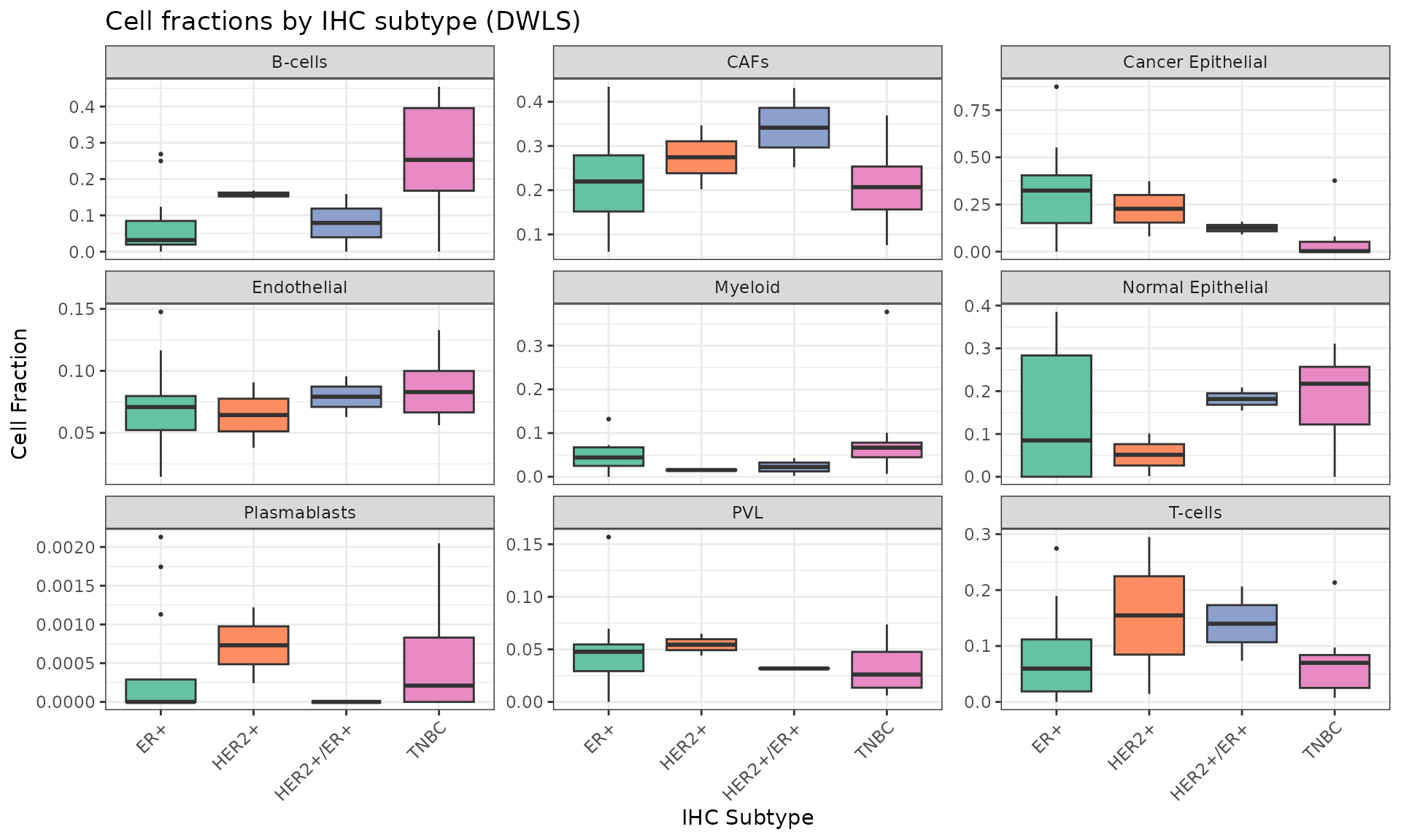
HER2-positive samples are enriched in T cells, while the ER-positive and triple negative breast cancer (TNBC) samples show an enrichment in cancer and normal epithelial cells, respectively. The patient metadata includes information about eventual treatments undergone by the patients. We can see that 5 out of the 24 patients were treated with Neoadjuvant and/or Paclitaxel, while the other 19 were untreated. We can therefore visualize the distribution of cell fractions across treated and untreated patients:

patients.results %>%
  filter(!is.na(Treatment)) %>%
  ggplot(aes(x = Treatment, y = cell_fraction, fill = Treatment)) +
  geom_boxplot(outlier.size = 0.5) +
  facet_wrap(~celltype, scales = "free_y", ncol = 3) +
  theme_bw() +
  theme(
    axis.text.x = element_text(angle = 45, hjust = 1),
    legend.position = "none"
  ) +
  scale_fill_brewer(palette = "Set1") +
  labs(
    x = "Treatment", y = "Cell Fraction",
    title = "Cell fractions by treatment status (DWLS)"
  )

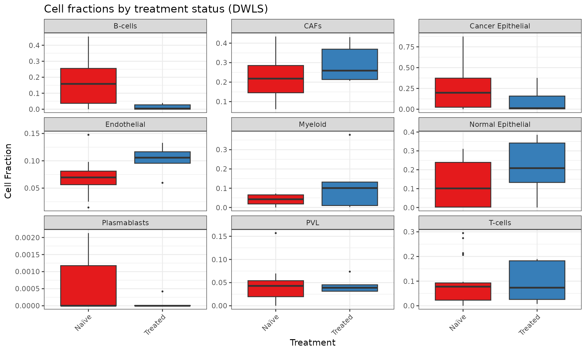
The major differences in this case are the enrichment of the CAFs and normal epithelial cells in the treated samples, as opposed to the cancer epithelial cells and B cells which have a higher median cell fraction in the untreated samples.

As mentioned before, with the lower level of annotations we can identify additional cell types, such as CD4+/CD8+ subtypes, Fibroblasts and cancer cells. We can therefore visualize the estimated cell fractions in a boxplot, focusing in particular on the CD4+ and CD8+ T-cell subtypes:

patients.results.minor %>%
  filter(celltype %in% c("T cells CD4+", "T cells CD8+"), !is.na(IHC_subtype)) %>%
  ggplot(aes(x = IHC_subtype, y = cell_fraction, fill = IHC_subtype)) +
  geom_boxplot(outlier.size = 0.5) +
  facet_wrap(~celltype, scales = "free_y") +
  theme_bw() +
  theme(
    axis.text.x = element_text(angle = 45, hjust = 1),
    legend.position = "none"
  ) +
  scale_fill_brewer(palette = "Set2") +
  labs(
    x = "IHC Subtype", y = "Cell Fraction",
    title = "CD4+ and CD8+ T-cell fractions by IHC subtype"
  )

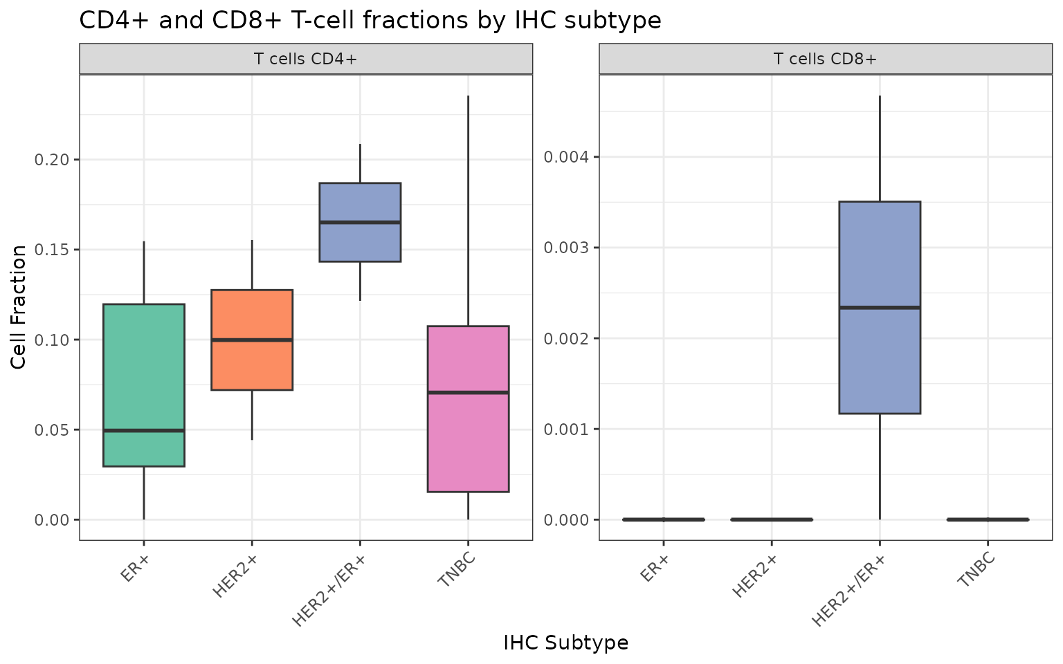
The estimates for the CD8+ T cells seem to be very low for all samples. On the other hand, in the HER2/ER positive samples the cell fractions estimated for the CD4+ T cells seem to be significantly higher than in the other subtypes.

Similarly, we can visualize the distribution of the estimates for the cancer associated fibroblasts (CAFs), respectively the myoblastic CAFs (myCAF) and the bone marrow derived inflammatory CAFs (MSC iCAF):

patients.results.minor %>%
  filter(celltype %in% c("CAFs myCAF-like", "CAFs MSC iCAF-like"), !is.na(IHC_subtype)) %>%
  ggplot(aes(x = IHC_subtype, y = cell_fraction, fill = IHC_subtype)) +
  geom_boxplot(outlier.size = 0.5) +
  facet_wrap(~celltype, scales = "free_y") +
  theme_bw() +
  theme(
    axis.text.x = element_text(angle = 45, hjust = 1),
    legend.position = "none"
  ) +
  scale_fill_brewer(palette = "Set2") +
  labs(
    x = "IHC Subtype", y = "Cell Fraction",
    title = "CAF subtype fractions by IHC subtype"
  )

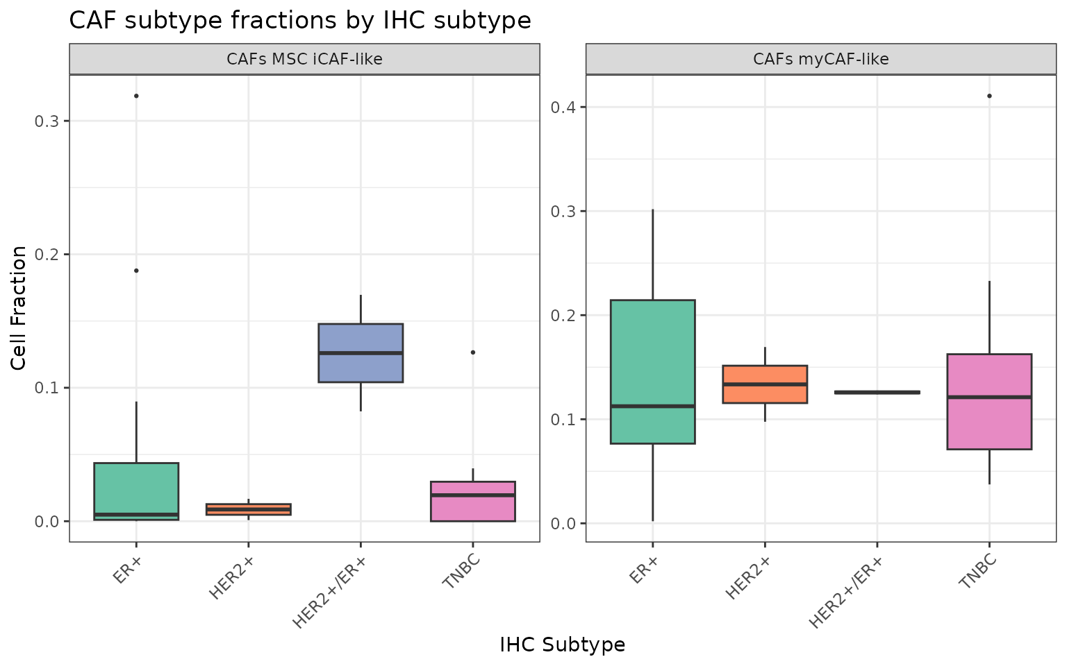
Here we can notice that, while the myoblastic CAFs have a comparable median value, the MSC CAFs have higher infiltration in the samples characterized as HER2+/ER+ subtype.

Finally, we can visualize the distribution of the different cancer cells molecular subtypes that were described by the authors:

patients.results.minor %>%
  filter(grepl("^Cancer", celltype), !is.na(IHC_subtype)) %>%
  ggplot(aes(x = IHC_subtype, y = cell_fraction, fill = IHC_subtype)) +
  geom_boxplot(outlier.size = 0.5) +
  facet_wrap(~celltype, scales = "free_y", ncol = 3) +
  theme_bw() +
  theme(
    axis.text.x = element_text(angle = 45, hjust = 1),
    legend.position = "none"
  ) +
  scale_fill_brewer(palette = "Set2") +
  labs(
    x = "IHC Subtype", y = "Cell Fraction",
    title = "Cancer cell subtype fractions by IHC subtype"
  )

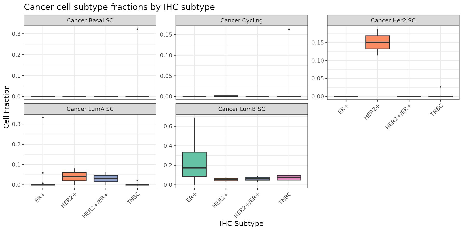
We can see that the HER2+ shows an overrepresentation of the cancer cells described as HER2-like by the authors. Similarly, the ER+ samples show higher fractions of Luminal B cancer cells. These findings on bulk RNA-seq are concordant with the subtypings that the authors described on the single cell RNA-seq (‘Results - scSubtype’).

References

Chu, Tinyi, Zhong Wang, Dana Pe’er, and Charles G. Danko. 2022. “Cell Type and Gene Expression Deconvolution with BayesPrism Enables Bayesian Integrative Analysis Across Bulk and Single-Cell RNA Sequencing in Oncology.” Nature Cancer 3 (4): 505–17. https://doi.org/10.1038/s43018-022-00356-3.

Finak, Greg, Andrew McDavid, Masanao Yajima, et al. 2015. “MAST: A Flexible Statistical Framework for Assessing Transcriptional Changes and Characterizing Heterogeneity in Single-Cell RNA Sequencing Data.” Genome Biology 16 (1). https://doi.org/10.1186/s13059-015-0844-5.

Hao, Yuhan, Tim Stuart, Madeline H. Kowalski, et al. 2023. “Dictionary Learning for Integrative, Multimodal and Scalable Single-Cell Analysis.” Nature Biotechnology 42 (2): 293–304. https://doi.org/10.1038/s41587-023-01767-y.

Heumos, Lukas, Anna C. Schaar, Christopher Lance, et al. 2023. “Best Practices for Single-Cell Analysis Across Modalities.” Nature Reviews Genetics 24 (8): 550–72. https://doi.org/10.1038/s41576-023-00586-w.

McDavid, Andrew, Greg Finak, Pratip K. Chattopadyay, et al. 2012. “Data Exploration, Quality Control and Testing in Single-Cell qPCR-Based Gene Expression Experiments.” Bioinformatics 29 (4): 461–67. https://doi.org/10.1093/bioinformatics/bts714.

Nault, Rance, Satabdi Saha, Sudin Bhattacharya, et al. 2022. “Benchmarking of a Bayesian Single Cell RNAseq Differential Gene Expression Test for Dose–Response Study Designs.” Nucleic Acids Research 50 (8): e48–48. https://doi.org/10.1093/nar/gkac019.

Tsoucas, Daphne, Rui Dong, Haide Chen, Qian Zhu, Guoji Guo, and Guo-Cheng Yuan. 2019. “Accurate Estimation of Cell-Type Composition from Gene Expression Data.” Nature Communications 10 (1). https://doi.org/10.1038/s41467-019-10802-z.

Wu, Sunny Z., Ghamdan Al-Eryani, Daniel Lee Roden, et al. 2021. “A Single-Cell and Spatially Resolved Atlas of Human Breast Cancers.” Nature Genetics 53 (9): 1334–47. https://doi.org/10.1038/s41588-021-00911-1.