Combined Methods Approach in deconvMe

The deconvolute_combined() function in deconvMe allows you to run multiple cell-type deconvolution methods simultaneously and create aggregated results. This approach can help reduce method-specific biases and provide more robust estimates of cell-type proportions.

Basic Usage

library(deconvMe)
library(minfiData)
options(matrixStats.useNames.NA = "deprecated")

# Example data
methyl_set <- minfiData::MsetEx

# Run multiple methods
result_combined <- deconvolute_combined(
  methyl_set = methyl_set,
  methods = c('epidish', 'houseman', 'methylcc'),
  array = '450k'
)

Understanding the Output

The combined results include both individual method results and aggregated estimates:

# View the structure
head(result_combined)

## # A tibble: 6 × 4
##   method  sample            celltype    value
##   <chr>   <chr>             <chr>       <dbl>
## 1 epidish 5723646052_R02C02 B cell      0.187
## 2 epidish 5723646052_R02C02 T cell CD4+ 0.199
## 3 epidish 5723646052_R02C02 T cell CD8+ 0    
## 4 epidish 5723646052_R02C02 other       0.185
## 5 epidish 5723646052_R02C02 Monocyte    0.306
## 6 epidish 5723646052_R02C02 Neutrophil  0

# Check available methods
unique(result_combined$method)

## [1] "epidish"    "houseman"   "methylcc"   "aggregated"

# Check available cell types
unique(result_combined$celltype)

## [1] "B cell"      "T cell CD4+" "T cell CD8+" "other"       "Monocyte"   
## [6] "Neutrophil"  "NK cell"

Cell-Type Standardization

The function automatically standardizes cell-type names across methods:

# Example of cell-type mapping
library(dplyr)

## 
## Attaching package: 'dplyr'

## The following objects are masked from 'package:dbplyr':
## 
##     ident, sql

## The following object is masked from 'package:minfi':
## 
##     combine

## The following objects are masked from 'package:Biostrings':
## 
##     collapse, intersect, setdiff, setequal, union

## The following object is masked from 'package:XVector':
## 
##     slice

## The following object is masked from 'package:Biobase':
## 
##     combine

## The following object is masked from 'package:matrixStats':
## 
##     count

## The following objects are masked from 'package:GenomicRanges':
## 
##     intersect, setdiff, union

## The following object is masked from 'package:GenomeInfoDb':
## 
##     intersect

## The following objects are masked from 'package:IRanges':
## 
##     collapse, desc, intersect, setdiff, slice, union

## The following objects are masked from 'package:S4Vectors':
## 
##     first, intersect, rename, setdiff, setequal, union

## The following objects are masked from 'package:BiocGenerics':
## 
##     combine, intersect, setdiff, setequal, union

## The following object is masked from 'package:generics':
## 
##     explain

## The following objects are masked from 'package:stats':
## 
##     filter, lag

## The following objects are masked from 'package:base':
## 
##     intersect, setdiff, setequal, union

# Show how cell types are mapped
cell_type_mapping <- data.frame(
  Original = c("CD8T", "CD4T", "B", "NK", "Mono", "Neu", "Unknown"),
  Standardized = c("T cell CD8+", "T cell CD4+", "B cell", "NK cell", "Monocyte", "Neutrophil", "other")
)
knitr::kable(cell_type_mapping, caption = "Cell-type standardization mapping")

Cell-type standardization mapping
Original	Standardized
CD8T	T cell CD8+
CD4T	T cell CD4+
B	B cell
NK	NK cell
Mono	Monocyte
Neu	Neutrophil
Unknown	other

The “Other” Category

The “other” category includes: - Cell types not in the standardized mapping - Method-specific cell types without equivalents - Rare or specialized cell populations

This category should be interpreted carefully, as it may represent: - True rare cell types - Method-specific artifacts - Incomplete cell-type coverage

Visualizing Combined Results

# Create visualization of individual vs aggregated results
library(ggplot2)

# Filter for one sample to show the comparison
sample_data <- result_combined[result_combined$sample == result_combined$sample[1], ]

ggplot(sample_data, aes(x = celltype, y = value, fill = method)) +
  geom_bar(stat = "identity", position = "dodge") +
  labs(title = "Individual Methods vs Aggregated Results",
       subtitle = paste("Sample:", sample_data$sample[1]),
       y = "Estimated Fraction",
       x = "Cell Type") +
  theme_minimal() +
  theme(axis.text.x = element_text(angle = 45, hjust = 1))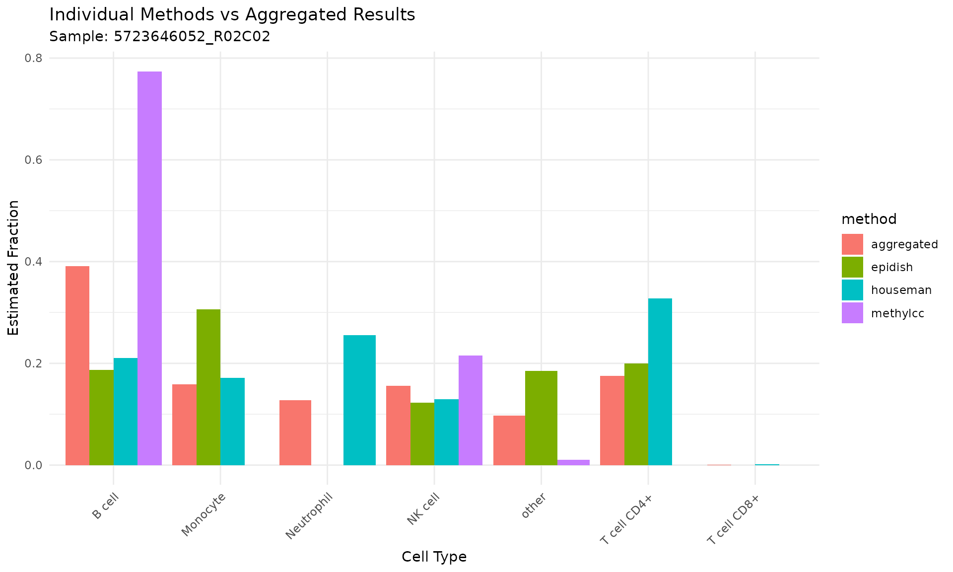

Limitations and Considerations

1. Method Heterogeneity

Different methods use different algorithms and reference datasets, which may not be directly comparable. Consider: - Whether methods are validated for your tissue type - The quality and relevance of reference datasets - Algorithm-specific assumptions

2. Equal Weighting

The current implementation gives equal weight to all methods. This may not be optimal if: - Some methods are more reliable for your specific use case - Methods have different levels of validation - You have prior knowledge about method performance

3. Missing Data

If a method fails to estimate a particular cell type, it may be excluded from aggregation, potentially biasing results.

4. Cell-Type Coverage

Methods may detect different sets of cell types, leading to incomplete coverage in aggregated results.

Quality Control

# Check for consistency across methods
consistency_check <- result_combined %>%
  group_by(sample, celltype) %>%
  summarise(
    mean_value = mean(value),
    sd_value = sd(value),
    cv = sd_value / mean_value,  # coefficient of variation
    .groups = 'drop'
  ) %>%
  filter(!is.na(mean_value))

# Identify cell types with high variability across methods
high_variability <- consistency_check %>%
  filter(cv > 0.5)  # arbitrary threshold